Building an EEG Event Classification System
From Raw Brain Signals to Deep Learning Predictions: A Complete Tutorial
Hands-on Tutorial: This article summarizes our open-source EEG classification project. All code, notebooks, and trained models are available in the GitHub repository. Clone it, run the notebooks, and experiment with your own data!
01Introduction to EEG Classification
Electroencephalography (EEG) is a non-invasive method of recording electrical activity in the brain. Clinicians use EEG to diagnose conditions like epilepsy, sleep disorders, and brain injuries by identifying specific patterns—called events—in the signal.
Manually reviewing hours of EEG recordings is time-consuming and requires expert knowledge. This is where machine learning comes in: we can train models to automatically detect and classify these events, assisting clinicians in their diagnostic workflow.
In this guide, we'll build a complete pipeline for EEG event classification using the Temple University Hospital (TUH) EEG Corpus—one of the largest publicly available EEG datasets. By the end, you'll have a working deep learning model that can classify EEG segments into different event types.
The Complete Pipeline
TUH Label Mapping
The TUH EEG Corpus uses a standardized labeling scheme across its datasets. Here's the complete mapping:
TUSZ / TUEV Labels (Events & Seizures)
| Code | Label | Description |
|---|---|---|
| 0 | NULL | Unlabeled / padding |
| 1 | SPSW | Spike and slow wave |
| 2 | GPED | Generalized periodic epileptiform discharge |
| 3 | PLED | Periodic lateralized epileptiform discharge |
| 4 | EYBL | Eye blink |
| 5 | ARTF | Artifact |
| 6 | BCKG | Background (normal activity) |
| 7 | SEIZ | Seizure (generic) |
| 8 | FNSZ | Focal non-specific seizure |
| 9 | GNSZ | Generalized non-specific seizure |
| 10 | SPSZ | Simple partial seizure |
| 11 | CPSZ | Complex partial seizure |
| 12 | ABSZ | Absence seizure |
| 13 | TNSZ | Tonic seizure |
| 14 | CNSZ | Clonic seizure |
| 15 | TCSZ | Tonic-clonic seizure |
| 16 | ATSZ | Atonic seizure |
| 17 | MYSZ | Myoclonic seizure |
| 18 | NESZ | Non-epileptic seizure |
| 19 | INTR | Interictal |
| 20 | SLOW | Slowing |
| 21 | EYEM | Eye movement |
| 22 | CHEW | Chewing artifact |
| 23 | SHIV | Shivering artifact |
| 24 | MUSC | Muscle artifact |
| 25 | ELPP | Electrode pop |
| 26 | ELST | Electrostatic artifact |
| 27 | CALB | Calibration |
| 28 | HPHS | Hyperventilation |
| 29 | TRIP | Photic stimulation |
TUAR Labels (Artifact Combinations)
| Code | Label | Description |
|---|---|---|
| 30 | ELEC | Electrode artifact |
| 31 | EYEM_MUSC | Eye movement + Muscle |
| 32 | MUSC_ELEC | Muscle + Electrode |
| 33 | EYEM_ELEC | Eye movement + Electrode |
| 34 | EYEM_CHEW | Eye movement + Chewing |
| 35 | CHEW_MUSC | Chewing + Muscle |
| 36 | CHEW_ELEC | Chewing + Electrode |
| 37 | EYEM_SHIV | Eye movement + Shivering |
| 38 | SHIV_ELEC | Shivering + Electrode |
02Loading EDF Files & Understanding EEG Data
EEG data is typically stored in EDF (European Data Format) files—a standard format for biosignal recordings. Each EDF file contains multiple channels of continuous voltage measurements sampled at a fixed frequency (commonly 250 Hz).
Loading with MNE-Python
The MNE-Python library provides robust tools for EEG analysis. Here's how to load an EDF file:
import mne

file_path = 'recording.edf'
raw = mne.io.read_raw_edf(file_path, preload=False)

# Access metadata
print(f"Channels: {raw.ch_names}")
print(f"Sampling frequency: {raw.info['sfreq']} Hz")
print(f"Duration: {raw.n_times / raw.info['sfreq']:.1f} seconds")
The 10-20 Electrode System
EEG electrodes are placed according to the 10-20 international system—a standardized arrangement ensuring consistent positioning across recordings. Each electrode has a name like FP1, C3, or O2:
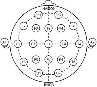
- Letters indicate brain region (F=frontal, C=central, T=temporal, P=parietal, O=occipital)
- Odd numbers are on the left hemisphere
- Even numbers are on the right hemisphere
- Z indicates the midline (zero)
Montage Transformation
Raw EDF files often store data in referential montage—each electrode measured against a common reference. However, clinical analysis typically uses bipolar montage, where adjacent electrodes are subtracted to highlight local differences.
Why bipolar? Bipolar montage reduces common noise and better localizes abnormalities. A spike appearing between two electrodes will show opposite deflections in adjacent channels.
# Transform to bipolar montage
# Example: FP1-F7 = FP1 electrode - F7 electrode
bipolar_data[0, :] = referential_data[fp1_idx, :] - referential_data[f7_idx, :]
The difference between referential and bipolar montage is clearly visible when visualizing the same recording:
data = raw.get_data()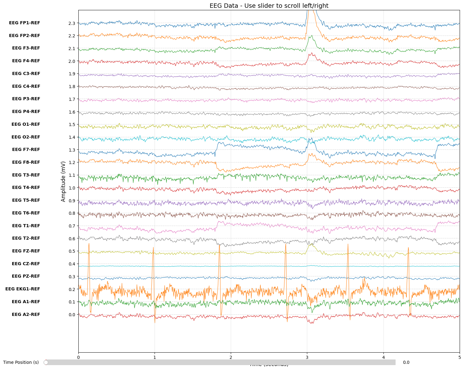
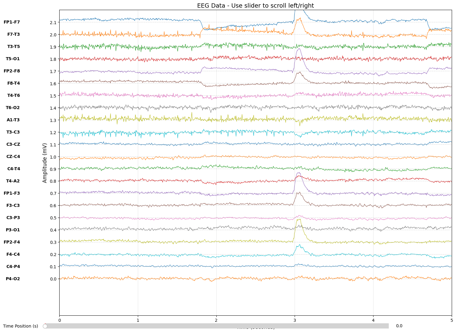
The TUH dataset uses a 22-channel TCP (Temporal-Central-Parietal) montage organized into chains:
| Chain | Channels |
|---|---|
| Left Temporal | FP1-F7, F7-T3, T3-T5, T5-O1 |
| Right Temporal | FP2-F8, F8-T4, T4-T6, T6-O2 |
| Left Parasagittal | FP1-F3, F3-C3, C3-P3, P3-O1 |
| Right Parasagittal | FP2-F4, F4-C4, C4-P4, P4-O2 |
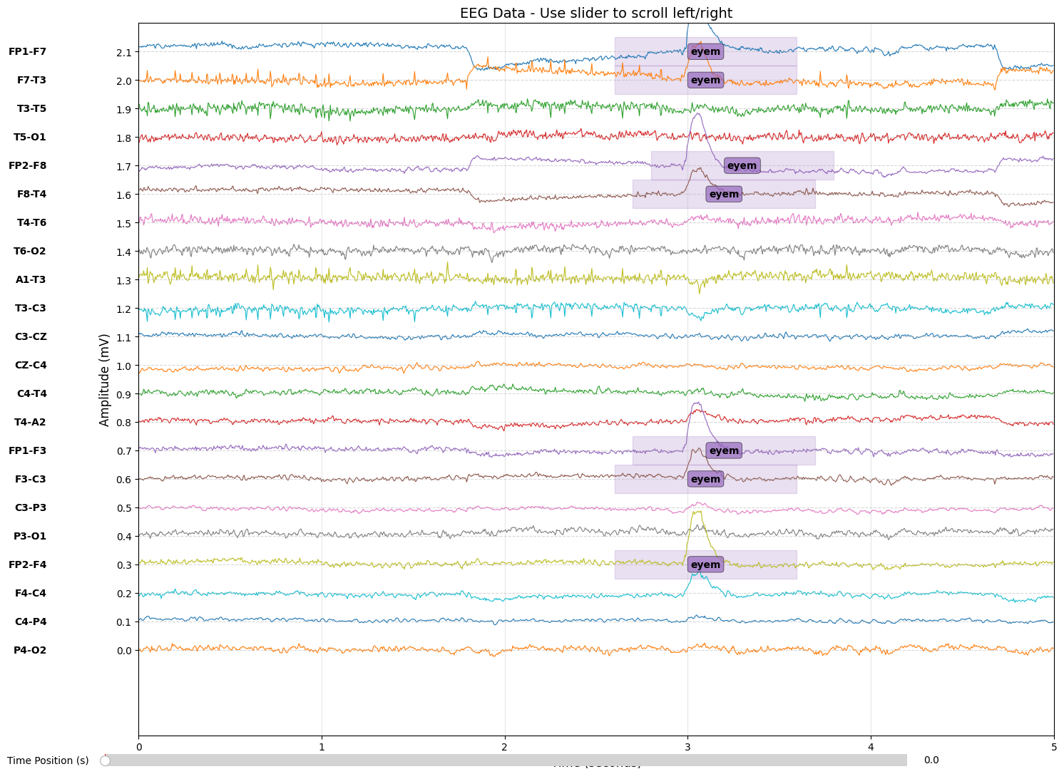
Loading Event Labels
The TUH dataset provides labels in .rec files (CSV format) alongside each EDF:
18,10.5,11.5,4    # channel, start_time, end_time, event_code
18,2.6,3.6,4
18,358.3,359.3,4
18,359.3,360.3,5
We convert these time-based annotations into a labels array matching the data dimensions—shape (n_channels, n_samples)—where each sample has an associated event code.
03Exploring Dataset Statistics
Before training a model, understanding your data distribution is crucial. The TUH EEG Corpus provides two complementary datasets with different annotation schemes. Note that we use only the 22-channel TCP montage described in the previous section across both datasets.
Background vs Unlabeled: These terms are often confused but have distinct meanings:
- Background (BCKG): An explicit label assigned by expert annotators indicating normal brain activity—the annotator reviewed the signal and confirmed nothing clinically significant is present. Serves as reliable "negative" examples for training.
- Unlabeled: Segments that haven't been reviewed at all—they could contain normal activity, artifacts, or clinical events, but we simply don't know. Should typically be excluded to avoid contaminating training with mislabeled samples.
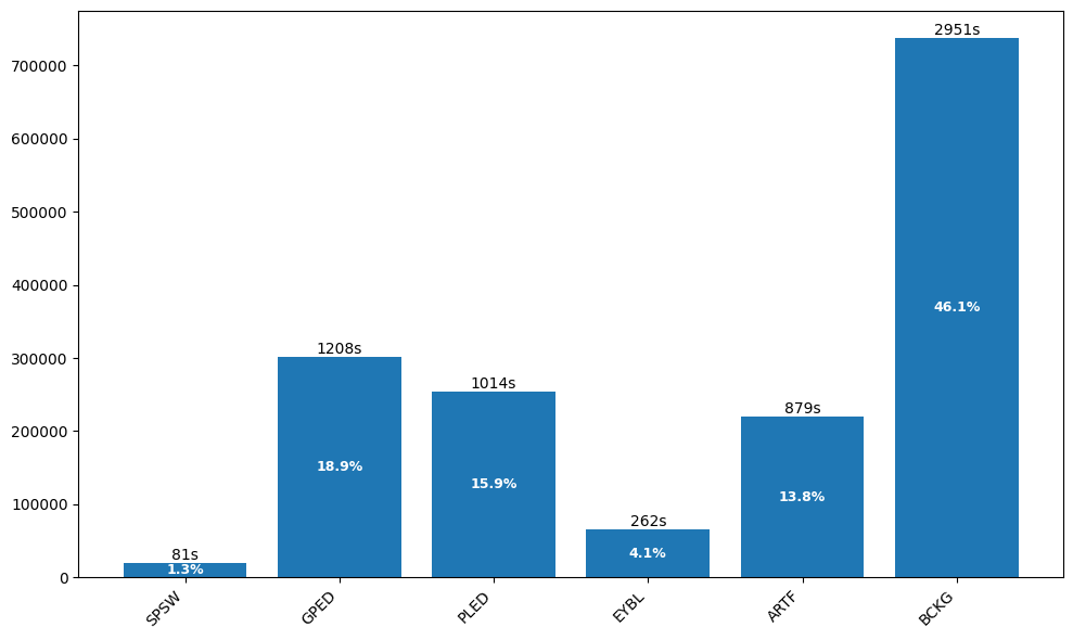
TUH EEG Events Distribution
The Events dataset contains 359 EDF files with annotations for six clinical event types. Background activity dominates, while clinically significant patterns like spike-and-wave are rare:
TUH EEG Artifacts Distribution
The Artifacts dataset contains 290 EDF files with fine-grained annotation of non-brain signals. Understanding artifact patterns helps build robust preprocessing pipelines:
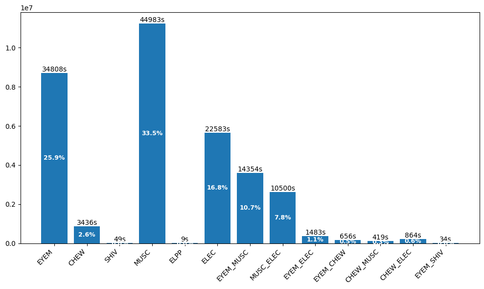
Class Imbalance Alert: Both datasets exhibit severe class imbalance. Rare but clinically important events like SPSW (1.3%) require careful handling during training—techniques like class weighting, oversampling, or focal loss can help.
04Preparing Data for Training
From this point on, we'll focus exclusively on the TUH EEG Events dataset. Our strategy is to split continuous EEG recordings into fixed-size windows for classification.
Windowing Strategy
We slice recordings into fixed-length windows (e.g., 1 second = 250 samples at 250 Hz). Key considerations:
- Filter unwanted labels: Skip windows containing only background/unlabeled segments
- Respect discontinuities: Only generate windows within contiguous valid segments
- Configurable overlap: Overlapping windows increase training data but risk data leakage
def window_generator(dataset, filter_labels, window_size_sec, overlap):
"""Generate windows from EEG data, avoiding discontinuities."""
for data, labels, metadata in dataset:
    window_size = int(window_size_sec * metadata['sfreq'])
    step_size = int(window_size * (1 - overlap))

    # Create mask for valid samples (not in filter_labels)
    mask = np.any(~np.isin(labels, filter_labels), axis=0)

    # Find contiguous segments using diff
    padded = np.concatenate([[False], mask, [False]])
    changes = np.diff(padded.astype(int))
    starts = np.where(changes == 1)[0]
    ends = np.where(changes == -1)[0]

    for seg_start, seg_end in zip(starts, ends):
        for win_start in range(seg_start, seg_end - window_size + 1, step_size):
            yield data[:, win_start:win_start + window_size], ...
Normalization
EEG amplitudes vary significantly across recordings, channels, and subjects. We apply z-score normalization per channel to standardize:
def normalize_window(data: np.ndarray) -> np.ndarray:
"""Z-score normalization per channel."""
eps = 1e-8
mean = data.mean(axis=1, keepdims=True)
std = data.std(axis=1, keepdims=True)
return ((data - mean) / (std + eps)).astype(np.float32)
Label Aggregation
Each window contains multiple sample-level labels. We use majority voting to assign a single label per window:
def majority_label_vote(labels: np.ndarray) -> int:
"""Return label if all samples identical, else 0 (mixed)."""
if labels.min() == labels.max():
    return int(labels.flat[0])
return 0  # Discard mixed-label windows
Prepared Dataset Summary
After windowing 359 EDF files with 1-second windows and no overlap:
| Class | Description | Windows | Percentage |
|---|---|---|---|
BCKG |
Background | 51,636 | |
ARTF |
Artifact | 10,118 | |
GPED |
Generalized Periodic Discharges | 8,805 | |
PLED |
Periodic Lateralized Discharges | 3,841 | |
EYEM |
Eye Movement | 655 | |
SPSW |
Spike and Wave | 397 | |
| Total | 75,453 | 100% | |
Preprocessing Tips
Before feeding EEG data into a model, consider these common preprocessing steps:
- Band-pass filter (0.5–50 Hz): Removes DC drift and high-frequency noise while preserving clinically relevant frequencies
- Notch filter (50/60 Hz): Eliminates power line interference (50 Hz in Europe, 60 Hz in North America)
- Amplitude clipping: Cap extreme values (e.g., ±500 µV) to reduce impact of movement artifacts and electrode pops
In this tutorial, we skip these steps to focus on the ML pipeline, but they can significantly improve model robustness in production.
05Training the Classification Model
With prepared data, we can now train a deep learning classifier. We use ResNet1D—a 1D adaptation of the popular ResNet architecture optimized for time series.
Class Remapping
To simplify our problem and address data scarcity in minority classes, we merge related events:
| Original | Mapped To | Rationale |
|---|---|---|
| SPSW (1) | Removed | Too rare (397 samples) |
| GPED (2), PLED (3) | Class 2: Periodic | Similar clinical patterns |
| EYEM (4), ARTF (5) | Class 1: Artifacts | Both are non-brain signals |
| BCKG (6) | Class 0: Background | Normal activity baseline |
This gives us a 3-class problem: Background, Artifacts, and Periodic Discharges.
Handling Class Imbalance
Even after remapping, background dominates. We apply random downsampling to balance:
# Before balancing:
# Class 0 (Background): 51,636
# Class 1 (Artifacts):  10,773
# Class 2 (Periodic):   12,646

dataset_balanced = downsample_class(dataset, class_to_downsample=0, target_count=13000)

# After balancing:
# Class 0: 13,000
# Class 1: 10,773
# Class 2: 12,646
Model Architecture
ResNet1D applies the residual learning framework to 1D convolutions:
| Parameter | Value | Description |
|---|---|---|
| Input | (1, 250) | Single channel, 1-second window |
| Base Filters | 32 | Scales up in deeper layers |
| Blocks | [2, 2, 2, 2] | ResNet-18 style architecture |
| Dropout | 0.2 | Regularization |
| Parameters | ~964K | Compact for EEG task |
Training Configuration
We use HuggingFace Trainer for a production-ready training loop:
training_args = TrainingArguments(
num_train_epochs=80,
per_device_train_batch_size=128,
learning_rate=0.0001,
weight_decay=0.01,
warmup_ratio=0.1,
lr_scheduler_type="cosine",

# Evaluation strategy
eval_strategy="steps",
eval_steps=200,
metric_for_best_model="f1_macro",
load_best_model_at_end=True,

# Logging
logging_steps=50,
report_to=["tensorboard"],
)
Metrics
For imbalanced classification, accuracy alone is misleading—a model predicting only the majority class would achieve 68% accuracy but be clinically useless. We track multiple metrics:
For our EEG classifier, we use F1 Macro as the primary model selection metric because it treats all classes equally—critical when rare events like SPSW (0.5% of data) are clinically important.
| Metric | What It Measures | When to Use |
|---|---|---|
Accuracy |
% of correct predictions overall | Only for balanced datasets |
Precision |
How many positive predictions were correct | When false positives are costly |
Recall |
How many actual positives were found | When missing cases is costly |
F1 Macro |
Average F1 across classes | Balance between precision and recall |
Training Results
After training on 29,135 samples with 7,284 validation samples:
- Model automatically saved with best F1 macro score
- Training progress visualizable via TensorBoard
- Checkpoints preserved for model recovery
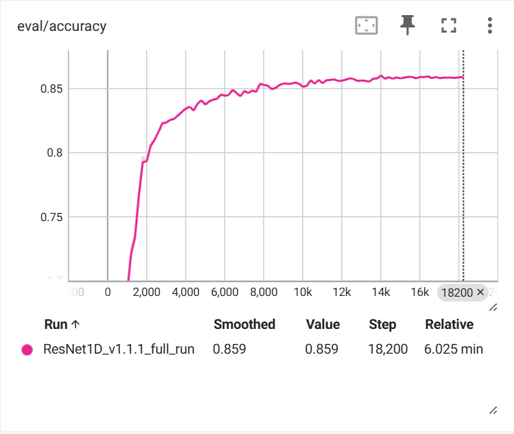
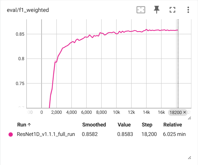
Training completed in approximately 6 minutes on GPU, demonstrating the efficiency of the ResNet1D architecture for EEG classification tasks.
More Metrics: Additional training metrics including loss curves, per-class precision/recall, and confusion matrices are available in the GitHub repository. You can visualize them locally by running tensorboard --logdir=runs/ after cloning the project.
06Conclusion & Next Steps
We've built a complete EEG event classification DEMO system from scratch:
- Data Loading: Parsed EDF files and transformed to bipolar montage
- Exploration: Analyzed dataset statistics and identified class imbalance
- Preparation: Windowed, normalized, and aggregated labels
- Training: Built and trained a ResNet1D classifier
The code and notebooks from this tutorial are available for educational purposes.